UTM zones with D3.js

I've just started to learn about the mapping capabilities of D3.js, and this is my first-ever D3.js visualization. I'm very impressed by the work on map projections by Jason Davies and Mike Bostock. It makes me believe that the Mercator renaissance will come to an end.

Mainland Norway is usually depicted in the Universal Transverse Mercator (UTM) projection. As the name implies, it's based on the cylindrical Transverse Mercator projection, which is supported by D3.js.

UTM is often used to show regions or countries with a greater north-south extent, like mainland Norway, which is usually depicted in UTM 33.

The UTM system divides the Earth between 80°S and 84°N latitude into 60 zones, each 6° of longitude in width. The zones are numbered from 1 to 60 proceeding east from the anitmeridian (180°). The projection has constant scale along the changing central meridian, and regions near it are mapped with low distortion. Just like on the regular Mercator projection, areas further away from the central meridian are increasingly distorted.

You can see it visualized in my rotating Transverse Mercator projection showing the 60 UTM zones around the Earth.

Converting shapefiles to TopoJSON + a GitHub secret

This blog post will show you how to convert shapefiles to TopoJSON. We'll convert the two shapefiles we created in my previous blog post, containing all counties and municipalities of Norway.

In a blog post from November last year I looked at various strategies to minify GeoJSON files. TopoJSON is an extension of GeoJSON that encodes topolog (e.g. shared borders between counties and municipalities). Polygons and lines in TopoJSON are represented by stiching together shared line segments. The shared boundary between two municipalities are represented only once, reducing the file size. Counties and municipalities are also sharing the same borders, and TileJSON are capeable of keeping both features in a single file. I won't go into detail, as the format is very well explained on this page.

Our shapefiles are using the Universal Transverse Mercator (UTM) 33N projection, a common projection for maps covering mainland Norway. If you want to keep this coordinate system in your TopoJSON file, you can just convert the shapefiles directly on the command line:

topojson --id-property NR -p name=NAVN -p name -o NO_Admin_UTM33.topojson NO_Fylker_pol.shp NO_Kommuner_pol.shp

You can download NO_Admin_UTM33.topojson on GitHub. As I want to show Norwegian counties and municipalities in various projections, I'm going to create a TopoJSON file with conventional latitude and longitude. Let's use QGIS to "unproject" our shapefiles:

• Add the shapefiles to a project.
• Right-click on the layer and select "Save As..."
• Choose a new filename.
• Click CRS Browse button and search for "EPSG:4326" (Filter). Select the CRS.
• Press OK.

You'll find "NO_Fylker_pol_latlng.shp" and "NO_Kommuner_pol_latlng.shp" on GitHub. If you open the files in QGIS you'll see that the shape of Norway is very different:

UTM 33 vs unprojected (latitude/longitude).

Let's convert the unprojected shapefiles to TopoJSON:

topojson --id-property NR -p name=NAVN -p name -o NO_Admin_latlng.topojson NO_Fylker_pol_latlng.shp NO_Kommuner_pol_latlng.shp

Cool! I knew that GitHub recently added support for GeoJSON, but you'll get an interactive map with TopoJSON as well! Just use .topojson as the file extension. Have a look at NO_Admin_latlng.topojson on GitHub. You can also embed the map on your page like this:



In the next blog post we're start mapping with D3.js. Let the fun begin!

Nice pile of wood on Foldøy island.

Splitting and clipping shapefiles with QGIS

In my last blog post, we improved a dataset containing all municipalities of Norway by merging polygons in QGIS. The municipality polygons include the sea areas, which makes it harder for people to recognize the shapes, as we're used to see Norway with all its fjords and islands. So let's use QGIS to remove the sea from all municipalities.

This is a two-step process. First we need to create a shapefile containing only sea areas. Let's open "NO_Arealdekke_pol.shp" in QGIS. This file contains land cover data, where one of the categories is sea areas ("Havflate").  

• Open the attribute table and select all sea areas (OBJTYPE = Havflate).  
• While the areas are selected, right-click on the layer name in the left column and select "Save Selection As...".
• Save the shapefile with a new name ("NO_Havflate_pol.shp"). 
• Open the new shapefile and click the "Toggle Editing" button.
• Mark all sea areas with "Select Features by Rectangle".
• Click the "Merge Selected Features" button.
• Save your changes. 
• You now have a shapefile with one large polygon of all sea areas in Norway. 

Next, we'll use our new shapefile to remove sea areas from the municipality dataset we created in the last blog post:

• Open both shapefiles in QGIS.
• In the main menu, select Vector -> Geoprocessing Tools -> Difference.
• Select the municipality dataset as "Input vector layer".
• Select the sea areas dataset as "Difference layer".
• Choose a new name for "Output shapefile".
• Press OK

We now have a new shapefile were the municipalities are only covering land areas. The clipping didn't work perfectly, and you'll se some parts left in the ocean. You can remove this line by clicking "Toggle Editing" and then on the "Delete Part" button. Click on the line in the ocean until all parts are removed.

The standard way to identify municipalties in Norway is four digit number, where the two first digits represent the county of the municipality. The dataset from the Norwegian Mapping Authority is missing leading zeros, which might give us problems when combining different datasets. We can use the Field Calculator in QGIS to add a new column with a 4 digits id:

You now have a shapefile with all the municipalities in Norway following the coastline. Finally I've merged all municipalities belonging to the same county to create a new shapefile of all the counties of Norway. You can download the shapefiles from GitHub ("NO_Kommuner_pol.shp" and "NO_Fylker_pol.shp").

Counties of Norway.

In the next blog post we're going to convert the shapefiles to TopoJSON, a compact vector format supported by D3.js. 

Kayaking around Foldøy island.

Merging polygons in QGIS

I'm going to play with the mapping capabilitites of D3.js in my new blog series from Foldøy island. I would like to use data from my own country, Norway. This dataset needs some improvements, and this blog post will show you how to do merge polygons in QGIS.

As announced in an earlier blog post, Norway will open it's topographic datasets to the public. This week we got some details about the launch:

• The data will be released on October 1st this year,
• The licence will be CC BY 3.0.
• Vector- and rasterdata at various scales up to 1:50,000 will be available. 
• This includes administrative borders for counties and municipalities and driveable roads longer that 50 meters. 
• Digital elevation data at 10x10 meter resolution, which is great news!

Before October 1st, I'm stuck with a dataset at 1:2,000,000 scale, but it will be suitable for country-wide mapping with D3.js. You can download the shapefiles from the Norwegian Mapping Authority on this page. 

This image shows the level of detail of the N2000 dataset from the Norwegian Mapping Authority. I've placed a small blue marker on Foldøy island, we're I'm currently staying. 

The dataset contains several shapefiles with point, line and polygon data. Let's open NO_AdminOmrader_pol.shp in QGIS: 

This shapefile contains polygons for all municipalities in Norway. If you open the attribute table you'll see that it's 430 features or municipalities, while the current numer is 428 (still far too many!). Municipalities in Norway are undergoing continuous consolidation, and this dataset is not up-to-date. January 1st this year, the municipality of Harstad and Bjarkøy was merged. Let's do the same in this dataset:

• Click on the "Toggle Editing" button.
• Open the attribute table and sort the municiaplities by name.
• Mark the municipality of "Harstad" and "Bjarkøy".
• Click on "Zoom map to the selected rows" if you want to locate the municipalities on the map.
• Click on the "Merge Selected Features" button.
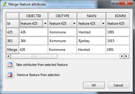
• Keep the attributes for Harstad. 
• In the attribute table, change the id ("KOMM") form 1901 to 1903. 

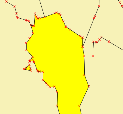
The former municipalities of Harstad and Bjarkøy in Northern Norway.

Remember to take the attributes form the correct feature while merging.

We still have one extra municipality, and this one is due to a bug in the dataset (UPDATE: This is not a bug, Sandefjord really has an enclave named Himberg in the neighbouring municipality. You should merge these two features into a multipolygon instead of the solution described below). The municipality of Sandefjord has two entries in the attribute table, and if you zoom to those features you'll see that Sandefjord has an enclave in the neighbouring municipaliy of Larvik:

The enclave of the municipality of Sandefjord.

This is sadly not the truth, let's get rid of the enclave:   

• Click on the "Select Single Feature" button.
• While pressing Ctrl-key select the enclave and the surrounding polygon. 
• Click on the "Merge Selected Features" button.
• Keep the attributes for Larvik.

Click on the "Save Edits" button, and you have a shapefile with the correct number of municipalties in Norway! You'll also find the shapefile on GitHub ("NO_AdminOmrader_pol.shp").

In the next blog post, we'll do some polygon clipping with QGIS.

Outdoor fireplace on Foldøy island - at midnight. 

Creating a synchronized view of two maps or images with Leaflet

In my last blog post, we created a Leaflet plugin capable of showing zoomable high-resolution images with Leaflet. Now, I need to compare two images side-by-side, and I've decided to create a generic plugin which can be used for maps as well.

The Leaflet.Sync plugin is just a few lines of code, but it took some time to figure out the inner workings of Leaflet. Here is a synchronized view of two maps of Foldøy island where I'm currently staying:

Fullscreen

This is the JavaScript code needed to create this map:

var layer1 = L.tileLayer('http://opencache.statkart.no/gatekeeper/gk/...'); 

var layer2 = L.tileLayer('http://opencache.statkart.no/gatekeeper/gk/...', {
    attribution: '© Kartverket'
});

var map1 = L.map('map1', {
    layers: [layer1],
    center: [59.336, 5.967],
    zoom: 14            
});

var map2 = L.map('map2', {
    layers: [layer2],
    center: [59.336, 5.967],
    zoom: 14,
    zoomControl: false                     
});

map1.sync(map2);
map2.sync(map1);

Create the maps as your normally do, and synchronize the maps with the sync method. You can synchronize one-way of two-way as above.

The plugin is not tested on different devices, so please report any issues on Github.

My new acquired friends on Foldøy. 

Showing Zoomify images with Leaflet

Today, I'm starting a new blog series written from Foldøy, a tiny island in south west Norway which will be my home for two months. In this first post, I'll show you how to deliver zoomable high-resolution images with Leaflet.

I've brought along 17 kg of mapping and visualization books to keep me occupied:


Fullscreen

Zoom in if you want to see the details! The photo is broken into tiles and then displayed as required. You don't really need Leaflet to create images like this, as Zoomify provides both Flash and HTML5 viewers. I decided to use Leaflet to create an open source alternative, and to learn more about tiling schemes.

This is the JavaScript code needed to show this image:

var map = L.map('photo').setView(new L.LatLng(0,0), 0);

L.tileLayer.zoomify('http://thematicmapping.org/playground/zoomify/books/', {
    width: 5472,
    height: 3648,
    tolerance: 0.8,
    attribution: 'Photo: Bjørn Sandvik'
}).addTo(map);

You have to provide the url to the Zoomify image folder and the with and height dimensions of the original image. You can also specify a display tolerance for the inital zoom level. A value lower than 1.0 might center the image and cut of the edges.

Image source: Microsoft Deep Zoom

The Zoomify tile format is similar to popular map tiling schemes, and I'm extending the Leaflet TileLayer class to show the image. The tiling follows a quadtree or pyramid pattern of increasing resolution, doubling the resolution for each zoom level. The tile size is 256 x 256 px and there are 256 tiles in each folder. The filename for each tile is z-x-y.jpg where z is the zoom level and x/y is the grid position starting from the top left corner.

The code is available on GitHub as a Leaflet plugin.

The bonfire is ready for midsummer on Foldøy island.

Fullscreen

You can create Zoomify tiles from your own image with Zoomify Express or from the Export menu in Photoshop.