Wednesday 25 July 2012

Creating contour lines with GDAL and Mapnik

Credits: Wikipedia
So far we’ve used our Digital Elevation Model (DEM) to create hillshade and color relief. Contours is another common cartographic method used to show the shape of the terrain. If contour lines are placed close to each other, it means that the terrain is steep. Let’s add some contours for our terrain map of Jotunheimen.

We can use a GDAL command, gdal_contour, to create vector contour lines from a DEM:

gdal_contour -a height jotunheimen.tif jotunheimen_contour_25m.shp -i 25.0

The resulting shapefile has an attribute named “height” (-a) containing the elevation of each contour line. The contour interval, the difference in elevation between successive contour lines, is 25 meters (-i).

Let's render the contour lines with Mapnik (jotunheimen_contours.xml):


We can use Nik2Img to create an image from the Mapnik XML file:

nik2img.py jotunheimen_contours.xml jotunheimen_contours.png -d 4096 4096 --projected-extent 460000 6810000 470000 6820000

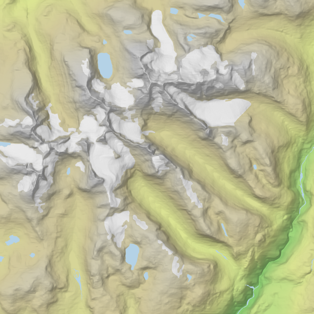
Contour lines for Besseggen mountain ridge

I want to render the contour lines differently for various zoom levels. The contours should be more visible at higher zoom levels, and we should add numbers showing the actual elevation for some of the contours. I also want to make the contour lines for every 100 meters thicker. To achieve this we need to know the map scale at different zoom levels. In the last blog post, we calculated the resolution (meters per pixel) for each zoom level. You get the map scale by dividing this number by 0.00028 (234.375 / 0.00028 = 837053.571).

Zoom
Resolution
Scale
0
234.375
837054
1
117.1875
418527
2
58.59375
209263
3
29.296875
104632
4
14.6484375
52316

For zoom level 4, the map scale is about 1:50,000. Read more about map scale on this excellent Mapnik page

Let’s create a style rule that will display the elevation on a contour line on zoom level 3:

If you look at the table above, the only scale number between the max and min scale denominator is 104632, which corresponds to zoom level 3. jotunheimen_contours2.xml includes all the style rules to render the contour lines differently for five zoom levels. You’ll also see that I’ve created contour shapefiles with contour intervals of 25, 100, 200 and 500 meters, - to be able to render these differently.

Finally, I've used TileCache to render transparent tiles with contours, and added them as a separate layer to Leaflet map:


Fullscreen map

Friday 13 July 2012

Using custom projections with TileCache, Mapnik and Leaflet

After five blog posts (1, 2, 3, 4, 5) we finally have a terrain map of Jotunheimen, a mountainous area in Norway with beautiful lakes and glaciers. It’s time to publish the map on the web. In this blog post I’ll show how you can use TileCache and Mapnik to render map tiles, and how to load these tiles into Leaflet using the UTM coordinate system.

To make a slippy map - a zoomable and draggable map - we need to serve map tiles instead of the large map image we created in the last blog post. The original Digital Elevation Model (DEM) is 3134 x 3134 pixels, and with a bit of upscaling we can using this tiling scheme:

Zoom
Map size
Tiles
Resolution
0
256 x 256 px
1 x 1 = 1
234.375
1
512 x 512 px
2 x 2 = 4
117.1875
2
1024 x 1024 px
4 x 4 = 16
58.59375
3
2048 x 2048 px
8 x 8 = 64
29.296875
4
4096 x 4096 px
16 x 16 = 256
14.6484375

Each map tile is 256 x 256 pixels. We need one map tile to cover the first zoom level and 256 tiles to cover the last zoom level. The original map area is 60.000 x 60.000 meters, and the resolution shows meters per pixel (60.000 / 256 = 234.375). We have enough information to configure TileCache (tilecache.cfg): 

[jotunheimen]
type=Mapnik
src=EPSG:32632
bbox=432000,6790000,492000,6850000
maxResolution=234.375                                       
mapfile=jotunheimen_terrain_ar50.xml

The bounding box for this map can be found here. jotunheimen_terrain_ar50.xml is the Mapnik configuration file we created in the last blog post. I’m also setting the cache type to GoogleDisk to store the tiles in Z/X/Y.png folders:

[cache]
type=GoogleDisk
base=/data/tiles

With tilecache_seed.py we can prerender the tiles automatically (zoom level 0 to 5):

tilecache_seed.py jotunheimen 0 5

We now have the map tiles on disk, and we can use Leaflet to create an interactive map:

var map = new L.Map('map', {
  crs:  L.CRS.proj4js('EPSG:32632', '+proj=utm +zone=32 +ellps=WGS84 +datum=WGS84 +units=m +no_defs', new L.Transformation(1, -432000, -1, 6850000)),
  scale: function(zoom) {
    return 1 / (234.375 / Math.pow(2, zoom));
  },
  layers: [
    new L.TileLayer('tiles/jotunheimen/{z}/{x}/{y}.png', {
      minZoom: 0,
      maxZoom: 4,
      continuousWorld: true
    }), 
    new L.Marker(new L.LatLng(61.636, 8.3135), {
      title: 'Galdhøpiggen 2469 m'
    })
  ],
  
  center: new L.LatLng(61.593, 8.397),
  zoom: 3,
  continuousWorld: true
});

The map is in UTM 32N projection (EPSG:32632). Using custom projections in Leaflet is not as easy as with OpenLayers, but Kartena is providing a great write-up of how it can be achieved. My map is combining Leaflet with Proj4js using the Proj4Leaflet bridge provided by Kartena. I've also added a marker for Galdhøpiggen, the highest mountain in Norway (2469 m).

This is what the map looks like:


Fullscreen map

Monday 2 July 2012

Land cover mapping with Mapnik

In the previous blog post we created a terrain map of Jotunheimen using color relief, hill and slope shading. All data originates from a single Digital Elevation Model (DEM). I miss two important features that dominates this area - lakes and glaciers. Let’s map it! The Norwegian Mapping Authority has not yet released detailed land cover data in the public domain. Low resolution data can be found on this page (scale 1:1,500,000). Luckily, I found the Corine Land Cover dataset (scale 1:100,000) from the European Environment Agency (EEA). Reuse for commercial or non-commercial purposes is permitted free of charge, provided that EEA is acknowledged. I downloaded two shapefiles from this dataset, 335 - Glaciers and perpetual snow and 512 - Water bodies. The Corine dataset is covering the whole of europe and use a different projection (EPSG:3035) than our map of Jotunheimen (EPSG:32632). Mapnik is able to clip and reproject vector data on-the-fly, so we can simply add the shapefiles to our Mapnik configuration file (jotunheimen_terrain3.xml):

I’ve added two styles for glaciers (white) and lakes (light blue) using the PolygonSymbolizer. The glacier layer is rendered on top of the color relief, before we blend it with with hill- and slopeshade layers. The lake layer is rendered on top of the blend. Since the shapefile and map projection is different, you have to specify the original projection in the srs attribute. Again, you’ll find the srs code by clicking on the Proj4 link on spatialreference.org.

Because of the large shapefiles, you need to specify the extent of the map 
(bbox) in the Python script that renders the image:

#!/usr/bin/env python
import mapnik
map = mapnik.Map(3134, 3134)
mapnik.load_map(map, 'jotunheimen_terrain3.xml')
bbox = mapnik.Box2d(mapnik.Coord(432000, 6790000), mapnik.Coord(492000, 6850000))
map.zoom_to_box(bbox)
mapnik.render_to_file(map, 'jotunheimen_terrain3.png')

The script will create this map image:

python jotunheimen_terrain.py


[ Download image ]
---
UPDATE 9 July 2012:
Viggo Lunde made me aware (see comment below) of a high resolution (scale 1:50,000) land cover dataset for Norway. The AR50 dataset (documentation) is available from the Norwegian Forest and Landscape Institute.
Jotunheimen is divided between two Norwegian counties - Sogn og Fjordane and Oppland. I downloaded the shapefiles for both counties and added them to jotunheimen_terrain_ar50.xml. The AR50 dataset contains many different land cover types, and I'm using filters in Mapnik to match styles to lake and glacier types:  <style name="glacier style"> <rule> <filter>[ARTYPE] = 70</Filter> <polygonsymbolizer fill="rgb(255,255,255)" /> </Rule> </style>
This image shows Hurrungane mountain range rendered with AR50 data:  
[ Download image ]
---

I’m quite happy with the result. In the next blog post we'll create an interactive version of this map.

Sunday 1 July 2012

Terrain mapping with Mapnik

In the previous posts we’ve created three different GeoTIFF images from a single Digital Elevation Model (DEM); hillshade, slopeshade and color relief. It’s time to combine the images into a single terrain map of Jotunheimen.


Mapnik is a great open source toolkit for map rendering, and we’ll use the RasterSymbolizer to blend the GeoTIFFs. The styles and layers (images) can be defined in an XML file (jotunheimen_terrain.xml):

The map projection (UTM 32N) is defined in the first line. Mapnik uses the PROJ.4 library, and you’ll find the srs code by clicking on the Proj4 link on spatialreference.org. Mapnik can’t alter the projection of raster images, so the images have to be in the desired projection before feeding them into Mapnik.

Next, I’ve defined two styles for this map with the RasterSymbolizer. The hillshade is going to be blended with the color relief image, using the multiply blend mode. The color numbers for each pixel of the hillshade are multiplied with the corresponding pixel for the shaded relief image. I’m also setting the opacity of the hillshade to 0.6, making it less dominant. The map layers are defined below the styles. Mapnik will render the layers in order, starting from the top.

You can use a simple Python script (jotunheimen_terrain.py) to render the map image (you can also use tools like TileCache and MapProxy):

#!/usr/bin/env python
import mapnik
map = mapnik.Map(3134, 3134)
mapnik.load_map(map, 'jotunheimen_relief.xml')
map.zoom_all() 
mapnik.render_to_file(map, 'jotunheimen_relief.png')

This script will create this PNG image:

python jotunheimen_terrain.py

[ Download image ]

Let’s add the slopeshade image to our XML file (jotunheimen_terrain2.xml):

I’ve adjusted the opacity of the slope- and hillshade to create this blend:

[ Download image ]

Which terrain map you prefer is a matter of personal preference. The first map has more glow on the light facing slopes. In the last map, the steep mountains are more defined and the light facing slopes are more detailed.

On both maps, I miss two important features for Jotunheimen - lakes and glaciers. Adding land cover data is the topic of the next blog post.